07_a_SamplingDistn.knit

---
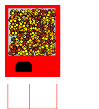
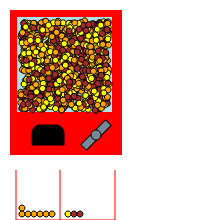
class: title-slide

# Samples, Statistics and their Distributions
## Dr. Uma Ravat
University of California at Santa Barbara

Copyright &copy; <a href="https://www.pstat.ucsb.edu/people/uma-ravat">Dr. Uma Ravat</a>
]

---
class: middle center
## Population and Sample
<img src="./img/pic-pop_sample.png" width="80%" style="display: block; margin: auto;" />

---
class: middle

The one million Reese's pieces candy in the candy machine
]

![](./img/pic-sample0.png)

A random sample of 10 Reese’s Pieces candies from the candy machine
]

---
class: middle center

![](./img/pic-candy_machine.png)

### I take a random sample of 10 Reese’s Pieces candies from  the machine, 3 times.

???

I get 3 samples each consisting of 10 Reese's Pieces

---
class: middle 
## Would you expect that I get

### these 3 samples

]
]

###  **OR** these 3 samples ?

]

---
class: center middle

## How variable are these samples ?

.left[
**Sampling variability: **
variability due to the sampling process which gives me different samples each time I sample.

]

---

# Quantifying sampling variability

---
class: middle

### How can we quantify sampling variability?

Describe each sample numerically.
 
----

--
### How can we describe each sample?

Count something about the sample 
 
----

--
### What can we count about each sample?

Proportion of orange candies in each sample of 10 Reese's pieces

???

- Need to quantify something about each random sample of 10 Reese's Pieces candies that I draw
- Convert each  sample into some sort of number
- Calculate the variance of that numeric

---
class: center top

# The proportion of orange Reese's pieces in the 3 samples

]

---
class: middle inverse
## Activity 1:  Take a random sample of 10 Reese’s Pieces candies from  the machine

### Let's all take one random sample!

1. Go [here](http://www.rossmanchance.com/applets/2021/oneprop/OneProp.htm?candy=1
)
2. In **Describe process:**
set Probability of orange  = 0.5, Number of candies = 10,  	Number of samples = 1 
2. In **choose statistic** in the middle left, select Proportion of orange
3. Click draw samples!
4. Put in the chat the value reported as  the Most recent `$\hat{p}$` in blue.

--
### Thank you all! You saved me a lot of work! 
- All your help is equivalent to "I take a random sample of 10 Reese’s Pieces candies from  the machine, **30 times**"
---
class: center split-six

I take a random sample of 10 Reese’s Pieces candies from the machine, ~~3~~ `30` times ?
 
]

.row[
<img src="./img/pic-sample-5.png" width="96" height="65">
<img src="./img/pic-sample-8.png" width="96" height="65">
<img src="./img/pic-sample-1.png" width="96" height="65">
]

.row[
<img src="./img/pic-sample-6.png" width="96" height="65">
<img src="./img/pic-sample-9.png" width="96" height="65">
<img src="./img/pic-sample-2.png" width="96" height="65">
]

.row[
<img src="./img/pic-sample-7.png" width="96" height="65">
<img src="./img/pic-sample-10.png" width="96" height="65">
<img src="./img/pic-sample-3.png" width="96" height="65">
]

---
class: middle

### How might we use this to quantify sampling variability?

--
   - standard deviation of the 30 numbers:  \{ 4/10, 6/10, 5/10, `$\cdots$` , 8/10\}

---
class: center

### Is there a better way to visualize the various proportions of orange candy we got in the 30 samples ?

---
class: middle

### Quantifying sampling variability SOLVED!

--
.pull-right[If we were to repeatedly take random samples of _fixed size_ from the population

#### We can use the standard deviation of the resulting sampling distribution of sample proportion to

- quantify sampling variability in our sampling procedure.

- [Aside] Looking at the mean of the resulting sampling distribution of sample proportion also provides key insights about the population.
]

---

If we were to repeatedly take random samples of _fixed size_ from the population.

- **varies** from sample to sample. 
- It is a **random variable**
- It has it's own distribution
    - The distribution of the proportion of orange Reese's pieces in repeated samples of _fixed size_ from the population of all candy in the machine.
]

--
.pull-right[
This distribution is called the **sampling distribution of sample proportion**

<img src="./img/visualizationOfsamplingdistn.png" width="300" height="220">Technically, this is actually an approximation of the theoretical sampling distribution.
]

---
class: middle inverse

# Group Activity 2: 
First Predict and then observe how the sampling distribution changes

Go [here](http://www.rossmanchance.com/applets/2021/oneprop/OneProp.htm?candy=1
)

_What would happen **to the sampling distribution of sample proportion** if.._

1. As the number of repetitions changes from **100** to **1000** to **10000** times while Drawing samples of size = 10, Probability = 0.5 remains fixed.
2. As you change the sample size to a few sizes from 25,50,100, 250 and  take repeated samples 100 times (optional 1000 times)  for Probability of orange = 0.5,
3. As you change the probability of orange to a few of 0.1,0.2,...,0.9 and take 100 repetitions  (optional 1000 repetitions) of samples of size 25, 50, 100,250.

- Let's simulate! 
- Be prepared to share your observations after simulation is done.

---
class: top

---
class: middle

### The sampling distribution of sample proportion

- is bell shaped for large sample sizes
- centered at the  population proportion
- as sample size increases, variance of this distribution decreases.

### You just discovered Central Limit Theorem !!!

---
class: inverse center middle

# Now, let's add all the math notation

--
to help succinctly describe the Central Limit Theorem you just discovered
---
class: middle

## Population Parameter and Sample Statistic

.pull-left[
- The population’s numerical characteristics are **parameters**. 
    - proportion of orange Reeses pieces in the candy machine is the population parameter `$p$`
    - `$p = 0.4$`
]

.pull-right[
- The sample’s numerical characteristics are **statistics**
    - proportion of orange Reeses pieces in the sample is the sample statistic `$\hat{p}$`
    - `$\hat{p} = 0.3$` 
]

- The distribution of the sample statistic is the **sampling distribution** **of the sample statistic**
    - the sampling distribution of the sample proportion (of orange candy)
    - the sampling distribution of `$\hat{p}$`
    - the sampling distribution (when the context is clear)
    
---
class: middle 
# Some more Terminology:

- The standard deviation of the sampling distribution is called the **standard error** denoted by **SE**
    - Sampling variability is just the standard error
    
- A sample statistic is also called a **point estimate of the population parameter**    
   - When we take a sample and calculate the sample proportion to get `$\hat{p} = 0.3$` then we say " 0.3  is a **point estimate** of the parameter `$p$`"

---
class: middle 
### Central Limit Theorem for sample proportions

Under certain conditions for sample size `$n$` and population proportion `$p$`*, the sampling distribution of sample proportion `$\hat{p}$` is

- approximately normally distributed 
- with mean equal to the population proportion, `$p$`, 
- standard error (SE) equal to `$\sqrt{\frac{p~(1-p)}{n}}$`.

$$ \hat{p} \sim \text{ approximately }N (mean = p , SE = \sqrt{\frac{p~(1-p)}{n}}) $$

- As sample size increases, standard error (variance) decreases
- For large sample sizes, `$\hat{p}$` will be close to true population proportion `$p$`.
- `$\hat{p}$` serves as a point estimate for `$p$`

---
class: middle 
# More sampling distributions and estimates for parameters

The strategy of using a sample statistic, and it's sampling distribution to estimate a parameter is quite common, and it’s a strategy that we can apply to other statistics besides a proportion. For example, the mean or average.

- Take a random sample of teenagers and ask them how many hours of sleep they got the previous night.
- Take the average hours of sleep in the sample. 
- Determine the sampling variability or SE of the sampling distribution of the sample mean
- Under certain conditions, CLT holds and we can use the sample average hours of sleep 
to estimate the average number of hours  that all teenagers sleep each night. 
- The details change only slightly.

---
class: middle 
# Central Limit Theorem for sample mean

For **any** population with population mean `$\mu$` and population variance `$\sigma^2$`, when sample size is large  ( `$n \geq 30$`), the sampling distribution of sample mean `$\bar{x}$` is

1. approximately normally distributed
2. with mean equal to the population mean `$\mu$`, 
3. standard error (SE) equal to `$\frac{\sigma}{\sqrt{n}}$`

$$ \bar{x} \sim N (mean = \mu, SE = \frac{\sigma}{\sqrt{n}}) $$
--

- Holds for [**any population**](https://onlinestatbook.com/stat_sim/sampling_dist/), even not normal, skewed etc.
- As sample size increases, standard error (variance) decreases
- For large sample sizes, `$\bar{x}$` will be close to true population mean `$\mu$`.
- `$\bar{x}$` serves as a point estimate for `$\mu$`

---
class: middle

## Recap: Central Limit Theorem (CLT)

For large sample sizes, the sampling distribution of sample means, sample proportions will be

1. approximately normally distributed 
2. with mean equal to the population parameter
3. The standard deviation will be inversely proportional to the square root of the sample size.

CLT allows us to make __inference__ about population parameters using sample statistics (also called point estimates).

---
class: middle inverse
### Activity 3:

The Youth Risk Behavioral Surveillance System (YRBSS) is a yearly survey conducted by the US Centers for Disease Control to measure health-related activity in high-school aged youth. The variables

- `age`: age in years
- `gender`: gender of participant, recorded as either `female` or `male`
- `grade`: grade in high school (9-12)
- `height`: height, in meters (1 m = 3.28 ft)
- `weight`: weight, in kilograms (1 kg = 2.2 lbs)

The CDC used the response from the 13,572 students to estimate the health behaviors of the target population: the 21.2 million high school aged students in the United States in 2013.

---
class: middle

1. Identify the population in this study. 
2. Identify the sample in this study.

- Population: the 21.2 million high school aged students in the United States in 2013.
- Sample: the responses received from the 13,572 students for each of the variables

Let's consider the random variable `weight`

- Are we given the population weights?
- Are we given the sample weights?
- Are we given the population mean weight `$\mu$`?
- Are we given the sample mean weight `$\bar{x}$`?

- To build the sampling distribution for sample average weight, we need to draw repeated samples of _fixed size_ from the population weights.

- Without knowing the population weights, how might we build the sampling distribution of sample average weight?

---
class: middle 
# Crucial note about real applications:

1. The population parameter is generally unknown
    - we used this information in building our sampling distribution
2. We have only one sample - the sample data that we observed/collected
    - we used several samples to building our sampling distribution

--
### Then how do we build our sampling distribution in real applications?
We need to understand how sampling distributions are used in statistics to _infer_ about the population (ie. make statements about population parameters)

---
class: middle 
###  The sampling distribution is never observed

-  Yet, it is useful to always think of a point estimate as coming from such a hypothetical distribution.

- In applications, the sampling distribution can be viewed as the result of asking the hypothetical question "What would the sampling distribution  look like if we took all possible samples of fixed size (= given sample size) if the population had _this particular parameter(s)_?"

- **_this particular parameter_** above is the value of the sample statistic calculated from the observed sample data.

---
class: middle

In the  Youth Risk Behavioral Surveillance System (YRBSS) example, from the 13,572 responses to the survey, we find that the average weight calculated from the sample data is about 68 kg.

For this YRBSS example, to determine the sampling distribution of sample average weight, we note that

- the sample size(13,572) is large, so CLT holds
- the sample average weight will be close to the unknown population weight
- This allows us to use the sample average weight of 68 kg as an estimate of the unknown population average weight.

---
class: middle

Then, to determine the sampling distribution of sample average, we would ask the hypothetical question,

- "What would the sampling distribution of sample average look like if we repeatedly took samples of size 13,572, from a population centered at 68 kg?"

From CLT, this sampling distribution

- would actually be approximately normal
- would be centered at 68 kg.
- The variance of the weights can also be estimated using the sample variance . 
- The standard error of the sampling distribution can then be estimated to be the `$\sqrt{\frac{\text{sample variance}}{13572}}$`.

---
class: middle 
## There are three distributions here

1. The population distribution 
    - generally unknown
2. The distribution of the sample 
    - known because we have observed data from one sample
3. The sampling distribution of the statistic 
    - under certain conditions, the sampling distribution is **known to be approximately** normally distributed from theory of mathematical statistics

---
class: middle

### Crucial Takeaways:

- The value of a (sample) statistic varies from sample to sample as we repeatedly take random samples from a population.
- Amazing that the long-run variability of sample meanss or  sample proportions  turns out (in many circumstances) to follow a beautiful **bell-shaped curve**!

---

# Acknowledgement

Thanks to Dr Mine Dogucu for suggestions for improvement of this material.

This content has been developed and shaped by referring to several materials including

1. [Dr. Allan Rossman's Ask good questions blog](https://askgoodquestions.blog/)
2. [OpenIntro.org resources](https://www.openintro.org/book/os/)
3. [Dr. Mine Dogucu materials](https://mdogucu.ics.uci.edu/l)

---
class: inverse center middle

# Next, let's flip things a bit